Architecture of a high performance GraphQL to SQL engine
Update: Tanmai spoke about this in more detail, including newer updates at the 2019 GraphQL Summit conference in SF.
The Hasura platform’s data microservice provides a HTTP API to query Postgres using GraphQL or JSON in a permission safe way.
You can exploit foreign key constraints in Postgres to query hierarchical data in a single request. For example, you can run this query to fetch “albums” and all their “tracks” (provided the “track” table has a foreign key to the “album” table):
{
  album (where: {year: {_eq: 2018}}) {
    title
    tracks {
      id
      title
    }
  }
}
As you may have guessed, the queries can traverse tables to an arbitrary depth. This query interface combined with permissions lets frontend applications to query Postgres without writing any backend code.
This API is designed to be fast (response time) and to handle a large throughput (requests per sec) while being light on resources (low CPU and memory usage). We discuss the architectural decisions that have enabled us to achieve this.
Query lifecycle
#
A query made to the data microservice goes through these stages:
Session resolution: The request hits the gateway which resolves the authorization key (if any) and adds the user-id and role headers and then proxies the request to the data service.
Query parsing: Data service receives a request, parses the headers to get the user-id and role, parses the body into a GraphQL AST.
Query validation: Check if the query is semantically correct and then enforce permissions defined for the role
Query execution: The validated query is converted to an SQL statement and is executed on Postgres.
Response generation: The result from postgres is processed and sent to the client (the gateway adds gzip compression if needed).
Goals
#
The requirements are roughly as follows:
The HTTP stack should add very little overhead and should be able to handle a lot of concurrent requests for high throughput.
Fast query translation (GraphQL to SQL)
The compiled SQL query should be efficient on Postgres.
Result from Postgres has to be efficiently sent back.
Processing the GraphQL request
#
These are the various approaches to fetch the data required for the GraphQL query:
Naive resolvers
GraphQL query execution typically involves executing a resolver for each field. In the example query, we would invoke a function to fetch the albums released in 2018 year and then for each of these albums, we would invoke a function to fetch the tracks, the classic N+1 query problem. The number of queries grows exponentially with the depth of the query.
The queries executed on Postgres would be as follows:
SELECT id,title FROM album WHERE year = 2018;
This gives us all the albums. Let the number of albums returned be N. For each album, we would execute this query (so, N queries):
SELECT id,title FROM tracks WHERE album_id = <album-id>
This would be a total of N + 1 queries to fetch all the required data.
Batching queries
Projects like dataloader aim to solve the N + 1 query problem by batching queries. The number of requests are not dependent on the size of the result set anymore, they’ll instead be dependent on the number of nodes in the GraphQL query. The example query in this case would require 2 queries to Postgres to fetch the required data.
The queries executed on Postgres would be as follows:
SELECT id,title FROM album WHERE year = 2018
This gives us all the albums. To fetch the tracks of all the required albums:
SELECT id, title FROM tracks WHERE album_id IN {the list of album ids}
This would be 2 queries in total. We’ve avoided issuing a query to fetch track information for each album and instead used the where clause to fetch the tracks of all the required albums in a single query.
Joins
Dataloader is designed to work across different data sources and cannot exploit the features of a single data source. In our case, the only data source we have is Postgres and Postgres like all relational databases provides a way to collect data from several tables in a single query a.k.a joins. We can determine the tables that are needed by a GraphQL query and generate a single SQL query using joins to fetch all the data. So the data needed for any GraphQL query can be fetched from a single SQL query. This data has be transformed appropriately before sending to the client.
The query would be as follows:
This file contains bidirectional Unicode text that may be interpreted or compiled differently than what appears below. To review, open the file in an editor that reveals hidden Unicode characters.
Learn more about bidirectional Unicode characters
This data has to be converted into JSON response with the following structure:
This file contains bidirectional Unicode text that may be interpreted or compiled differently than what appears below. To review, open the file in an editor that reveals hidden Unicode characters.
Learn more about bidirectional Unicode characters
We discovered that most of the time in handling a request is spent in the transformation function (which converts the SQL result to JSON response). After trying few approaches to optimise the transformation function, we’ve decided to remove this function by pushing the transformation into Postgres. Postgres 9.4 (released around the time of the first data microservice release) added json aggregation functions which helped us push the transformation into Postgres. The SQL that is generated would become something like:
This file contains bidirectional Unicode text that may be interpreted or compiled differently than what appears below. To review, open the file in an editor that reveals hidden Unicode characters.
Learn more about bidirectional Unicode characters
The result of this query would have one column and one row and this value is sent to the client without any further transformation. From our benchmarks this approach is roughly 3–6x faster than the transformation function in Haskell.
Prepared statements
#
The generated SQL statements can be quite large and complicated depending on the nesting level of the query and the where conditions used. Typically any frontend application has a set of queries which are repeated with different parameters. For example, the above query could be executed for 2017 instead of 2018. Prepared statements are best suited for these use cases, i.e when you have complicated SQL statements which are repeated with a change in some parameters.
So, the first time this GraphQL query is executed:
{
  album (where: {year: {_eq: 2018}}) {
    title
    tracks {
      id
      title
    }
  }
}
We prepare the SQL statement instead of executing it directly, so the generated SQL will be (notice the $1):
This file contains bidirectional Unicode text that may be interpreted or compiled differently than what appears below. To review, open the file in an editor that reveals hidden Unicode characters.
Learn more about bidirectional Unicode characters
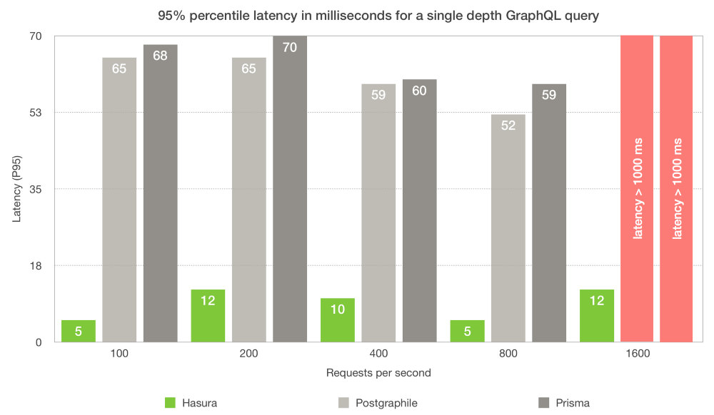
All these optimisations put together result in some serious performance benefits. Here’s a comparison of Hasura’s architecture with Prisma and Postgraphile.
Hasura’s GraphQL API compared with Postgraphile and Prisma. This post was first published in April 2018 and these benchmarks are from older versions of Prisma & Postgraphile. Performance optimizations have since gone into all the projects featured below.
In fact, the low memory footprint and negligible latency when compared to querying postgres directly, you could even replace the ORM with GraphQL APIs for most use-cases on your server-side code.
Benchmarks:
Details of the setup:
An 8GB RAM, i7 laptop
Postgres was running on the same machine
wrk was used as a benchmarking tool and for different types of queries, we tried to “max” out the requests per second
A single instance of the Hasura GraphQL engine was queried